Chapter 2 – Data curation
Outline
Part 2B – 2D classification
-
- What is 2D classification and why do we do it?
- Practical advice & guidelines
- Hands-on
Part 2C – Particle dataset curation
- Practical advice & guidelines
- Hands-on
In Chapter 1, we discussed the Preprocessing steps for processing your cryo-EM dataset, walking you through motion correction, CTF estimation, and particle picking. In this Chapter, we will discuss how to curate your particle stacks to give you the best stack for subsequent 3D analysis jobs. This will include micrograph curation, 2D classification approaches to remove ‘bad’ particles, and strategies for cleaning particle stacks with 2D classification and particle selection.
Part 2A – Micrograph curation
Why does micrograph curation matter?
As the adage goes, “Garbage-in, garbage-out.” In cryo-EM, this adage relates to micrograph quality: bad micrographs entering analysis will lead to bad results. To give an example, here is an example dataset of a GPCR membrane protein complex:
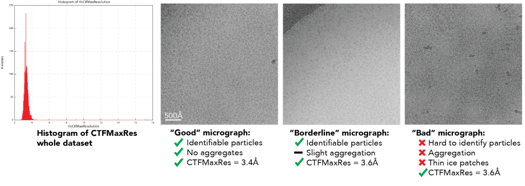
The dataset was collected on a Titan Krios using a direct electron detector. Analysis of the CTFMaxRes plot from CTFFIND4 and RELION shows that >99% of the dataset has CTFMaxRes below 4Å.
Upon closer inspection, we could see at least three general categories of micrographs:
- “Good” – these micrographs have clear particles that were evenly distributed
- “Borderline” – these micrographs have some clearly identifiable particles, but alongside, there were small aggregates/aggregates
- “Bad” – these micrographs showed clumped, aggregated particles.
Notably, all of these micrographs have CTFMaxRes values lower than 4Å, which is due to the high quality of the imaging instrument and the large amount of sample per image. This means that using a CTFMaxRes cutoff won’t eliminate these bad micrographs.
What is so bad about including bad micrographs?
In processing this dataset, if you were to ‘only’ curate using CTFMaxRes as the metric for removing micrographs after particle picking and 2D classification, you would get these class averages:
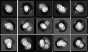
These class averages are ‘bad’ because:
- There is no secondary structure seen in any class average
- All of the averages show a ‘fuzziness,’ which is due to particle misalignment
- Some of the averages show stippling, which is caused by overalignment of noise.
Now, instead of using CTFMaxRes for curating micrographs, we used a tool in the Cianfrocco Lab called “MicAssess,” which is a deep-learning-based neural network that we trained to learn what are good and bad micrographs. We trained MicAssess on ‘good’ and ‘bad’ micrographs from in-house and EMPIAR datasets.
After removing bad micrographs from this GPCR dataset using MicAssess, we re-processed the data and were able to obtain much-improved results:
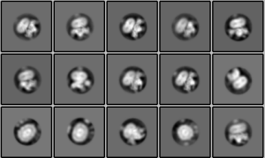
These class averages represent ‘good’ class averages for the following reasons:
- Secondary structure is seen in both the transmembrane helices and peripheral membrane proteins
- The protein density looks smooth with no stippling
Overall, we hope this shows you that curating cryo-EM micrographs is critical for robust downstream analysis results.
Primary literature:
-
- High-Throughput Cryo-EM Enabled by User-Free Preprocessing Routines. Li Y et al. 2020 Structure. PMID: 32294468.
- IceBreaker: Software for high-resolution single-particle cryo-EM with non-uniform ice. Olek M et al. 2022. Structure. 2022 35150604.
- Review: What Could Go Wrong? A Practical Guide to Single-Particle Cryo-EM: From Biochemistry to Atomic Models. Cianfrocco & Kellogg. 2020. J Chem Inf Model PMID: 32078321.
Additional online content:
What is a ‘bad’ micrograph?
Bad micrographs are any micrographs that don’t have your sample of interest – there are many ways to find bad micrographs on any grid!
To start, here is a gallery of ‘good’ micrographs:
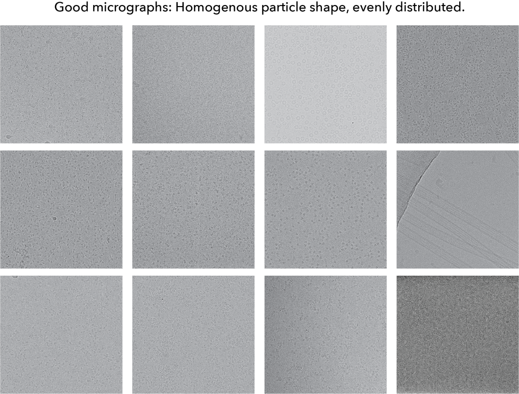
The main take-home points for this gallery:
- Particle shape – when looking at any given micrograph, the particles all look similar. There aren’t wide variations in the size or spread across a micrograph
- Particle distribution – the particles are spread nearly evenly across the micrograph. Importantly, the particles are dense. The bottom right image shows a very dense image of a membrane protein.
- Defocus – The defocus is between 0.5 – 2 microns. Low defocus data will be easier to analyze later given that high defocus data will require much larger box sizes.
Next up, here is a gallery of ‘bad’ micrographs:
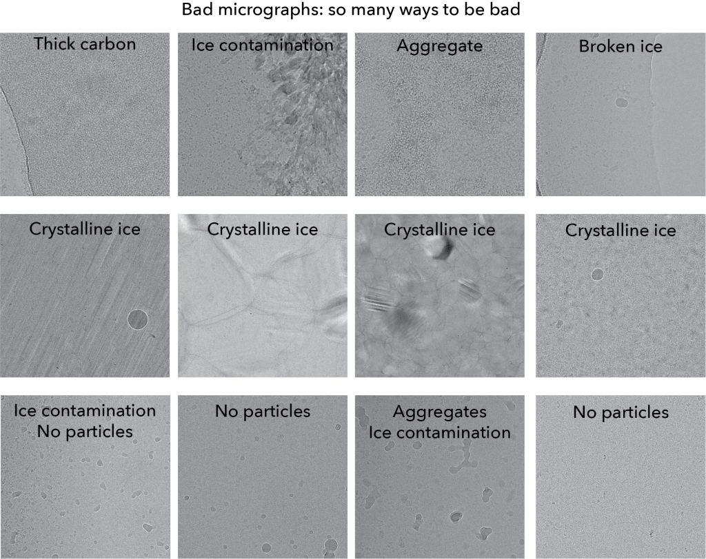
For each micrograph, we label what the ‘diagnosis’ of what make it bad. You’ll see that there is a range of ways to be bad: no particles to aggregates, thick carbon to broken ice.
What you should keep in mind is how will you remove these types of bad micrographs? Below, in practical advice, we will outline the best approaches to remove these micrographs in datasets.
Additional online content:
Practical advice & guidelines on micrograph curation
Below, we will outline categories of ‘bad’ micrographs and strategies to remove them from your dataset. We have grouped them into bins that are 1) straightforward, 2) challenging, or 3) require manual intervention to remove bad micrographs.
How will I know what ‘kind’ of bad micrographs are in my dataset??
Unfortunately, you will need to look at many of your micrographs using visual inspection to get a sense of what issues you have in your dataset. We recommend thumbing through all of your dataset quickly to see what data is in it.
Straightforward curation
The following metrics will be covered in this section and should always be used for micrograph curtation:
- CTFMaxRes
- Relative ice thickness
- Defocus range limits
Here is a description of bad micrograph categories and solutions to remove the bad micrographs:
- Empty micrographs
- Problem: There is nothing in the micrograph because the image was taken over an empty hole.
- How to remove from the dataset: CTFMaxRes or the confidence of the CTF fit will be an effective way to remove this from your dataset. When nothing is in the micrograph, no CTF can be fit. This will lead to a very low-resolution CTFMaxRes and low confidence in the CTF fit.
- Broken ice
- Problem: The micrograph shows strong movement due to ice breaking/micrograph moving during exposure.
- How to remove from the dataset: Given that part of the image will be empty (broken micrograph) and/or the micrograph is showing movement during the exposure, you can remove this type of micrograph by setting a CTFMaxRes cutoff. You will need to explore what this value is for your dataset, but typically, setting a limit of 6Å (where micrographs >6Å are removed) should remove this type of micrograph.
- Crystalline ice
- Problem: The micrograph shows crystalline ice due to slowed freezing, whereby the particles in the micrograph are not in vitreous ice. You can tell that a micrograph has crystalline ice by seeing white/black banding patterns in the micrograph or seeing reflections in the power spectrum at the ~3.7Å resolution shell.
- How to remove from the dataset: These micrographs will have a strong signal in Fourier space at the water ring (~3.7Å). Both cryoSPARC and RELION-5+ provide a metric of “ice thickness,” which is a relative measure of the water ring intensity versus background intensity in the power spectrum.
- Too low / too high defocus:
- Problem: Particles are not visible in the micrograph due to a low defocus, or the particles are very contrasted due to a high defocus (>5 microns).
- How to remove from the dataset: After CTF estimation, you should look at the distribution of estimated defocus values. Look at the micrographs with the lowest estimated defocus – can you see particles? If not, keep looking at micrographs to determine the lowest defocus where it is possible to still see your particles. If your eye can’t see the particles, neither will the particle picking programs! Next, look at the high defocus estimated micrographs. In this case, you should just remove all micrographs with a defocus greater than 5 microns. High defocus may increase contrast of particles, but it comes at the cost of large delocalized signal, which will require a very large box size for high-resolution structure determination.
Challenging curation
For this set of bad micrographs, you should expect to dig into optimizing several aspects of preprocessing and curation. The following suggestions will vary per sample and dataset but should provide a general overview of how you’d go about removing these micrographs.
- No particles
- Problem: There is vitreous ice, but there are no particles in the micrograph
- How to remove from the dataset: Two strategies to remove these kinds of micrographs, and you may need to employ both:
- CTFMaxRes – Identify the micrographs that do not have particles. What is the CTFMaxRes? Is there a clear difference in the value of CTFMaxRes for these no-particle micrographs versus your micrographs that have particles? If so, then use this metric.
- Number of particles picked – In principle, if you have already identified a robust particle-picking approach for your dataset, these micrographs without particles should have different particle-picking behavior. Compare the number of particles picked for empty micrographs versus your good micrographs – can you use a minimum or maximum number of particles picked per micrograph to exclude these micrographs that are missing particles (but have vitreous ice)?
- Ice contamination (non-crystalline)
- Problem: Your micrographs have circular, hexagonal, or amorphous ice contaminants. They sometimes may even look like a protein sample.
- How to remove from the dataset: Depending on the severity of the contamination, you have two choices:
- Particle picking – If you can tune your particle picking, you may be able to avoid these contaminants effectively. These contaminations usually have higher scoring values with templates or template-free picking, which means you may be able to set an upper threshold for the particle-picking program to avoid ice.
- Manual curation – If particle picking doesn’t work, you may need to manually go through your dataset to identify contaminated images and remove them from your dataset. Typically these images will have normal CTFMaxRes and relative ice thickness, so it can be hard to remove other than manual inspection.
Require manual intervention or MicAssess
Below are categories of bad images that cannot be easily removed with the basic statistics provided by cryoSPARC or RELION. They need to be removed through manual inspection or by running a visual curation tool such as MicAssess.
- Aggregates
- Problem: Some micrographs show large aggregates of your protein sample.
- How to remove from the dataset: These aggregates are hard to remove given that they will have a good CTFMaxRes (since there is a lot of the sample in the image for CTFMaxRes signal) and the relative ice thickness will be within a reasonable range. You should explore whether particle picking is sensitive to these aggregated images and investigate if any trends could be used to remove these. Next, you should poke around your dataset to see how much is aggregated. If a lot of it is aggregated, then you should consider 1) manual curation and/or 2) collecting a new dataset without as much aggregation. Finally, if you really want to process this dataset, try using a program like MicAssess to remove the aggregated micrographs.
- Thick carbon/gold
- Problem: Some micrographs in your dataset were from mis-targeting during data collection and have thick carbon/gold foil in most of the micrograph.
- How to remove from the dataset:
- Thick carbon – Thick carbon will have a very high CTFMaxRes since there is so much signal from the carbon. You will have to determine if particle picking can sort this otherwise you will need to find these manually. Ideally, this should not comprise a lot of your dataset if data collection went without much issue.
- Gold foil – Gold foil from UltrAuFoil or HexAuFoil grids should have a lower CTFMaxRes than good micrographs, given that most electrons will not be able to scatter through the gold foil (i.e., the gold strongly scatters the electrons).
Please submit any suggestions or comments to cryoedu-support [at] umich.edu.