Chapter 1 – Preprocessing
Outline
Part 1A – Motion correction
Motion correction aims to estimate and remove sample movement from the movies in a cryo-EM dataset.
Understanding raw cryo-EM data
Raw cryo-EM data corresponds to a stack of movie frames, where each movie frame is a sparse image consisting of zeros and ones. The movie data are collected using direct electron detectors, a class of detectors that identify each electron as it interacts with the detector, localizing the electron to a specific pixel.
Here is an example of a micrograph shown alongside a single frame:
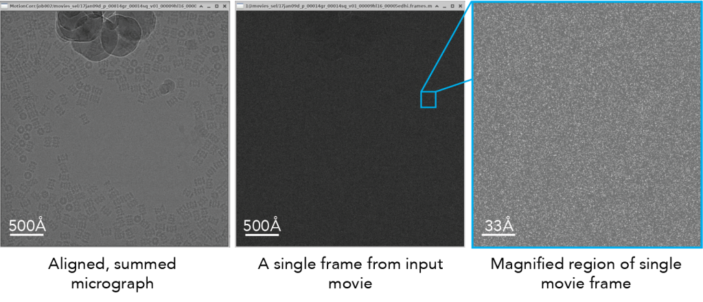
Notice that when we magnify the raw frame, you can see individual counts on the electron detector (right): white spots correspond to ‘counted’ electrons whereas dark gray areas are pixels without any detected electrons.
Primary literature:
- Electron counting and beam-induced motion correction enable near-atomic-resolution single-particle cryo-EM. Li et al. 2013 Nature Methods PMID 23644547.
- Review: Direct Electron Detectors. McMullan, Faruqi, Henderson. 2016. Methods Enzymology PMID 27572721.
Additional online content:
Importing data into RELION
To perform motion correction on a complete dataset, you first need to import all of the movies into RELION. In this video, we will show you how to log into the cryoEDU cloud desktop and import data into RELION:
Motion correction
Motion correction refers to the process of computationally aligning frames together in a cryo-EM movie to remove as much motion as possible, ultimately producing a single aligned, summed, micrograph. This example shows the effect of sample motion on a plunge-frozen cryo-EM viral sample:

Figure reference: Brilot et al. 2012.
The image on the left (A) is a summed movie without alignment whereas the image on the right (B) is the same movie but using frame alignment. The aligned micrograph shows sharper images of the viral particles.
Sample motion is due to a drumming motion, where compression forces for the thin film of water and the support film are released when electrons hit the sample (see figure, below). This ‘buckling’ of holes is directly related to the thickness of the ice relative to the thickness of the hole. As such, it is possible to select a hole size that prevents large sample movements. In this figure, the authors demonstrate that thin films of samples will not have movement if the hole diameter is ~300 nm. This observation led to the development of 300 nm ‘HexAuFoil’ grids, which are grids that do not have beam-induced movement.
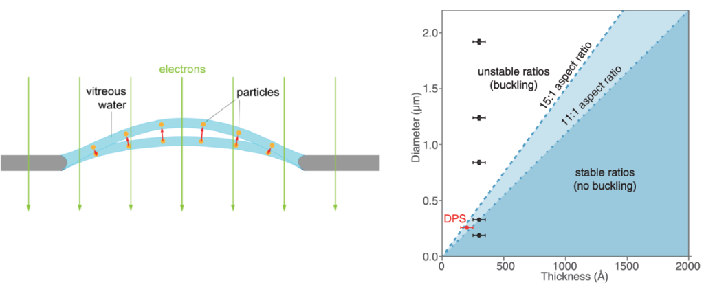
Figure reference: D’Imprima et al. 2021, Naydenova et al. 2020.
Motion correction is typically performed using patches of the movie to locally correct the motion of exposure. Early work in cryo-EM benefited from using global motion correction, where entire frames were aligned together to produce a motion-corrected output image (e.g., Li et al. 2013 using ‘MotionCorr’ software). Since this initial work performing global motion correction, the field has moved towards patch-based motion correction. In this approach, individual patch motion trajectories are combined with global motion in addition to the trajectories of neighboring patches to provide a significantly improved alignment of patches during the movie exposure.
An example of patch-based motion correction is shown here. The global trajectory of the frames is shown as the enlarged line, whereas the motion of local patches are shown within dotted boxed outlines. Note that the lines indicate motion (X vs. Y movement) over time (blue > white > red). Since this original algorithm in ‘MotionCor2,’ other software programs such as RELION and cryoSPARC have adopted comparable patch-based motion correction.

Figure reference: Zheng et al. 2017.
Why can’t we perform per-particle motion correction at this stage? You may be wondering this question – why use patches if we can select particles and then align every particle across the movie frames? It turns out that most single particles exhibit much too noisy trajectories that are challenging to fit accurately. To deal with per-particle motion, 3D references must be used. This will be covered in Chapter 3.
Primary literature:
- Beam-Induced Motion of Vitrified Specimen on Holey Carbon Film. Brilot et al. 2012. J. Structural Biology PMID 22366277.
- MotionCor2: anisotropic correction of beam-induced motion for improved cryo-electron microscopy. Zheng et al. 2017. Nature Methods PMID 28250466.
- Electron cryomicroscopy with sub-Ångström specimen movement. Naydenova et al. 2020. Science PMID 33033219.
Additional online content:
- ‘Motion Correction’ on cryoEM101.org.
- ‘MyScope’ training on Motion Correction (Microscopy Australia).
- SBGrid Webinar: MotionCor2 & AreTomo by Shawn Zheng.
Running motion correction in RELION:
Gain reference
Cryo-EM direct electron detectors can have pixels with different sensitivities to electrons. This variation can introduce artifacts into the images, affecting the accuracy of the structural information obtained from the sample. A gain reference is a calibration tool used to correct for variations in the sensitivity of the detector across its surface and it is applied to our data during the motion correction job.
The gain reference is an image of the detector without a sample. This image captures how each pixel in the detector responds to a uniform input signal. When you use a gain reference, you divide the raw images obtained during your experiments by the gain reference image. This process normalizes the response across the detector, correcting for pixel-to-pixel variations. As a result, the corrected images more accurately represent the sample, improving the quality of the data for subsequent analysis and reconstruction of the molecular structure.
Here is an example of a gain reference.
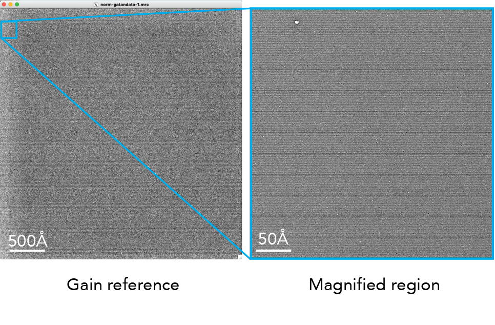
Unfortunately, you will need to experimentally determine how to apply the gain reference to your movies. Due to camera and software conventions, gain references are sometimes saved in an orientation that is opposite from your data. This means you need to rotate or flip X/Y the gain reference to find the appropriate orientation. The only way to know it worked is to look at the output micrograph (see below for example).
Incorrectly applying gain references will lead to artifacts in the output aligned micrograph. Depending on your detector, you may or may not be able to easily tell the difference. In the above example, it is challenging to visually determine if the gain reference was correctly applied.
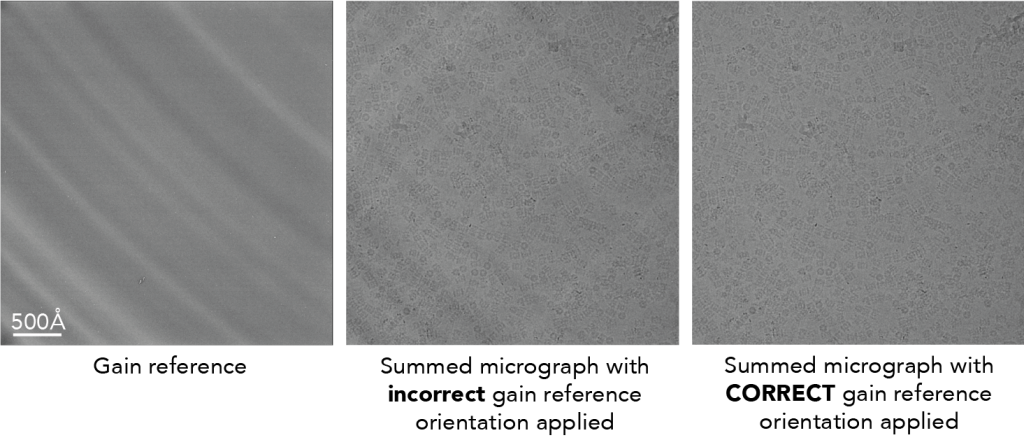
To highlight what it could look like, here is an image from a different dataset (EMPIAR-10025) that shows more strong features on the detector. The image of the gain reference is shown on the left. The radial patterns are caused by back thinning of the support matrix to increase the precision of marking an electron hitting the detector (e.g., see Figure 3 in McMullan et al. below). You can see that when the gain reference is incorrectly applied, the resulting micrograph shows both dark and white patterns streaking across the image (middle). These patterns go away when the orientation is correctly specified (right).
Primary literature:
- Experimental observation of the improvement in MTF from backthinning a CMOS direct electron detector. McMullan et al. 2009 Ultramicroscopy PMID 19541421.
Wait, why aren’t the movies stored in a gain-corrected format?
We store our movies in raw format (i.e., not gain corrected) to save on disk space for the movies. Since we count individual electron events on the detector, each pixel only has whole numbers (‘integers’) for each pixel on each frame. In this format, the movies are stored as 8-bit values. Then, once gain corrected, the micrographs as stored as 16-bit files. When we gain correct, the process of subtracting the gain reference from the aligned micrograph causes the numbers to be stored as numbers with decimal values (‘float’ values). Changing the original integer values to float values increases the bit-depth of the movie, which increases the file size. This is why we only store movies in integer format whereas micrographs are float format.
Oh no! I’ve lost my gain reference file
Not to fear – you can estimate the gain reference from your dataset. Since the gain reference is constant in a raw cryo-EM dataset, if you sum all the frames from all the movies in a dataset you will ‘only’ see the gain reference. RELION has a tool to estimate the gain reference: relion_estimate_gain.
Dose weighting

Practical guidelines for motion correction & dose weighting
General tips:
- Use patch-based motion correction
- Use all frames (i.e., don’t throw out the first or last frames)
- Use positive Bfactors during alignment (100-500Ų). This is a type of lowpass filter to dampen high-resolution information during alignment.
- Float16 – this option will save micrographs with a lower bit depth and save storage space.
- Perform dose weighting
- Bin super-resolution movies back to the physical pixel size (this also saves space). You can find out if your data is super-resolution by looking at the image dimensions. The physical pixel dimensions is ~4000 x 4000 pixels whereas super-resolution will be ~8000 x 8000 pixels.
RELION – Motion correction
- Save sum of of power spectra: Yes. This will generate a summed power spectrum that comes from summing the individual power spectra of each frame. Due to water molecules moving during the exposure, these summed power spectra will be different than summing all frames in real space and then taking power spectra. See McMullan et al. 2015 for more details.
- Number of patches: For rectangular detectors (e.g., Gatan K3) – use 5 x 7 patches; For square detectors using 5 x 5.
- Binning factor – if you collected movies in super-resolution mode, bin the data back to the physical pixel size by including a value of ‘2’.
cryoSPARC – Patch motion correction
- Output F-crop factor – if you collected movies in super-resolution mode, bin the data back to the physical pixel size by indicating 1/2.
Hands on:
Process RELION or cryoSPARC tutorial data:
- Can you see differences in the output summed micrographs if you do/do not apply a gain reference?
- What is the most number of patches that you can use and see a difference in the output?
- What happens if you increase or decrease the Bfactor? What if you make the Bfactor negative?
Interactive online resources:
- Google Colab Notebook: Run RELION motion correction on EMPIAR-10025 T20S proteasome movies.
- cryoEDU RELION simulator
Part 1B – CTF estimation
Contrast Transfer Function (CTF) estimation aims to measure the optical aberrations in cryo-EM micrographs. This information is saved and used in later steps (e.g., 2D/3D classification, 3D refinement) for CTF correction.
What is the CTF?
There are several excellent resources to describe this in more detail (see links below). But, briefly, the CTF is a function that describes the oscillations in Fourier space that are caused by micrographs being out of focus. For instance, here is the 2D power spectrum (the Fourier transform of a micrograph squared) of a micrograph:
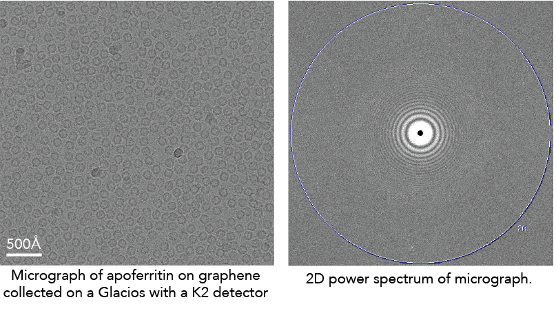
The CTF describes the oscillating dark/white patterns in the power spectrum. These aberrations act as a complicated band-pass filter that allows us to see the particles. If the micrograph was taken close to focus, the particles will become nearly invisible.
Primary literature:
- Accurate determination of local defocus and specimen tilt in electron microscopy. Mindell & Grigorieff. 2003. Journal of Structural Biology. PMID: 12781660.
- CTFFIND4: Fast and accurate defocus estimation from electron micrographs. Rohou & Grigorieff. 2015. Journal of Structural Biology. PMID: 26278980.
- Gctf: Real-time CTF determination and correction. Zhang. 2016. Journal of Structural Biology. PMID: 26592709.
Additional online content:
- cryoSPARC – CTF estimation
- cryoEM101.org – CTF estimation
- CTF estimation and restoration – Himes & Grigorieff
- Grant Jensen – CTF correction
- Wikipedia – Contrast transfer function
Interactive:
CTF estimation: RELION + CTFFIND4/Gctf
Running the job
- Input micrographs STAR: Micrographs from motion correction.
- Use micrograph without dose weighting: Yes. Dose weighting changes the appearance of Thon rings, so it’s better to use the un-dose weighted micrograph.
- Program choice: CTFFIND4.1 or Gctf. Both programs are OK for CTF estimation. The major difference is how they are run and output information. CTFFIND4 runs on CPUs whereas Gctf runs on GPUs. Practically, it may be harder to run Gctf because it runs on older GPU CUDA libraries. CTFFIND4 is a much more well-tested program than Gctf which is what the Cianfrocco lab uses.
- Use power spectra from MotionCorr job: Yes. Using the summed power spectra will be faster (no Fourier transforms required of the entire micrograph) and more accurate because the Thon rings will be more visible.
Other parameters: During CTF estimation, CTFFIND4/Gctf will cut out a smaller region from the micrograph for the Fourier transform (FFT box size) and then fit the CTF function within defined regions of Fourier space (Minimum and Maximum resolution) using a fixed search range of defocus values (Minimum and Maximum defocus) with a given defocus step size. The only parameters to consider changing would be the defocus range if you know that you have data with higher defocus than 5 microns.
Interpreting the results
RELION will output a logfile.pdf that you should inspect. This helps you see the defocus range and quality of fit parameters for the CTF estimation step. When RELION is running CTF estimation, it is running CTFFIND4/Gctf directly on the command line and then taking output parameters from these jobs and incorporating them into the output files. Here is what an example output looks like CTFFIND4 when you run CTFFIND4 without RELION:
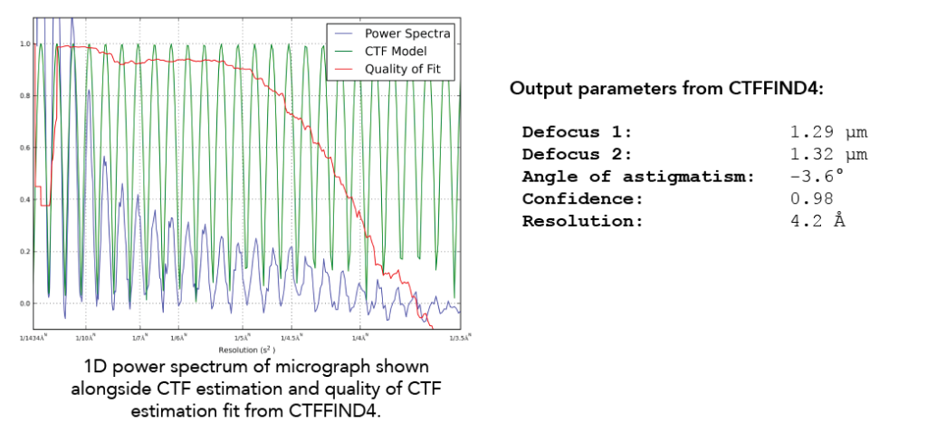
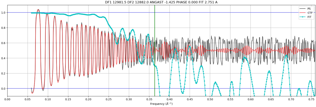
Parameters output from CTFFIND4 include the defocus in both X & Y directions, the angle of astigmatism, the confidence of the fit, and the resolution. The two values for defocus and the angle of astigmatism allow CTF correction programs to accurately define the astigmatism (if any) in a given micrograph. This information is used to create a 1D power spectrum of the micrograph (blue curve), which collapses the 2D power spectrum into a single axis. On this same plot is shown the CTF model based on the fitting (green) (Note that there are no negative values here given that the X-axis is squared reciprocal space). Finally, CTFFIND4 uses the experimental power spectrum and the fit to calculate a confidence score (red). The X-axis resolution number is recorded when the confidence dips below a specified threshold at 0.5. This is known as CTF Maximum Resolution.
To assess your datasets, it is critical to examine the collective statistics of defocus and CTF Maximum Resolution. We always examine these statistics and then remove micrographs based on defined limits for defocus and CTF maximum resolution. In RELION, you can use the Subset selection option in the GUI to remove micrographs with rlnCtfMaxRes values worse than 6Å. In cryoSPARC, under the Exposure curation > Manually curate exposures, you can select micrographs with CTF maximum resolution below a set value (e.g., 6Å).
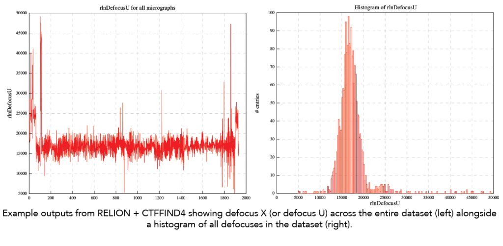
- Defocus range: Below is an example output from RELION run with CTFFIND4 showing the range defocus estimates from a dataset in the Cianfrocco lab. Note that the range is not very wide, which may affect downstream resolutions of reconstructions later. Moreover, ideally, the defocus should be closer to 1 micron defocus instead of centering on ~1.8 microns defocus.
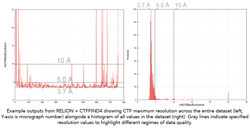
- CTF Maximum resolution: Here is the trace of CTF maximum resolution values for a given dataset. Note that the goal is always to have CTF maximum resolution values below 4Å to ensure optimal contrast of particles and data quality. The ability to fit the CTF to below 4Å indicates enough protein and signal to high resolution. For traditional single particle datasets, seeing CTF maximum resolution fits worse than 4Å is likely a sign that it will be challenging to go to high resolution due to too thick ice. In this example below, we see that the ‘best’ data is at ~3.7Å and then there are also micrographs with a CTF maximum resolution ~5Å. As an end user, you should look at the micrographs in these different categories to see if they are different. The 5Å fit is likely from micrographs with thicker ice.
Primary literature
- Thon rings from amorphous ice and implications of beam-induced Brownian motion in single particle electron cryo-microscopy. McMullan et al. 2015. Ultramicroscopy. PMID: 26103047.
Additional online content
CTF estimation: cryoSPARC – Patch CTF estimation
Running the job
We recommend Patch CTF estimation, which estimates the local defocus variations across a given micrograph.
- Input: Micrographs from motion correction
- Other parameters: Number of micrographs to plot – increase this number if you want to see plots from more than 10 micrographs. You may also need to increase the upper defocus limit if your dataset has micrographs with a defocus of more than 4 microns.
Interpreting the results
cryoSPARC will show plots for the number of micrographs indicated above. Here are the plots and a description of what they show.
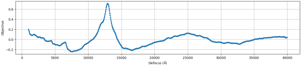
- CTF objective function fitting: This plot shows the resulting score (Y axis) as a range of defocus values (X axis) are compared with a given micrograph. High confidence estimates will have a single, sharp peak, indicating that the algorithm found the solution. If this plot appears flat or multiple peaks, there is likely something wrong with your data.
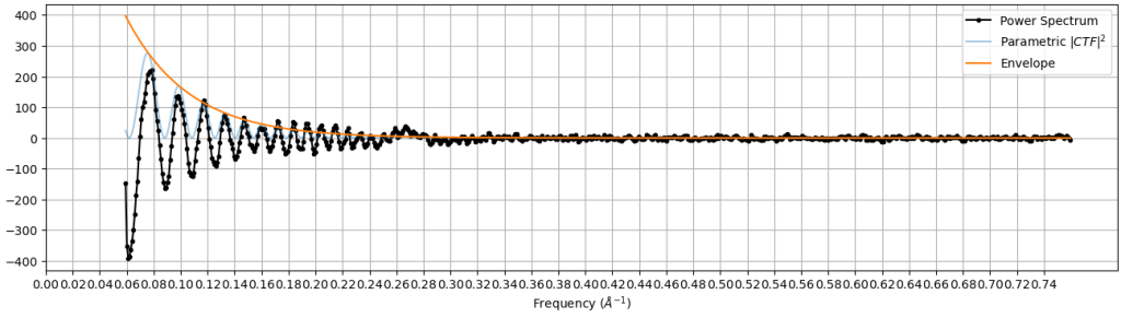
- Comparison of measured CTF versus power spectrum: This plot shows the experimental power spectrum (black) superimposed with the estimated CTF function (light blue). The X axis is Fourier space and the Y axis intensity. These two plots should have the same peak locations. The orange line is the envelope of the CTF estimation, which describes the decay of high resolution signal at higher resolutions.
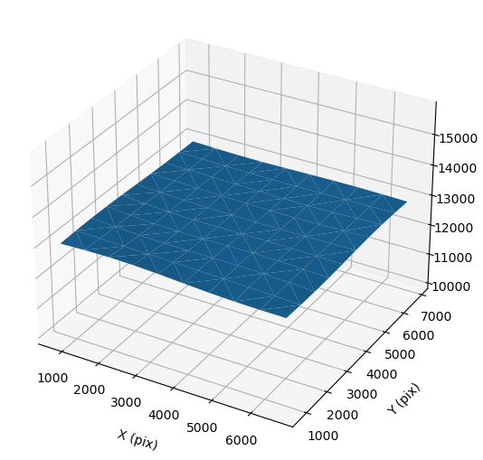
- 2D plot of defocus versus position on micrograph: This 2D plot shows the defocus (Z axis) versus position on the micrograph (X & Y axes). For an untilted micrograph like this, the plot is generally flat. Tilted samples will have a consistent angle across the sample.
- Quality of CTF fit: This plot shows the experimental power spectrum (black) versus the measured CTF (red) across a range of spatial frequencies (X axis). The Y axis shows the correlation between the experimental and measured CTF. At low spatial frequencies, there is very good agreement (correlation = 1). At higher frequencies, these plots start to disagree, which is shown with a lower correlation. The fit resolution is marked where confidence drops below 0.5.
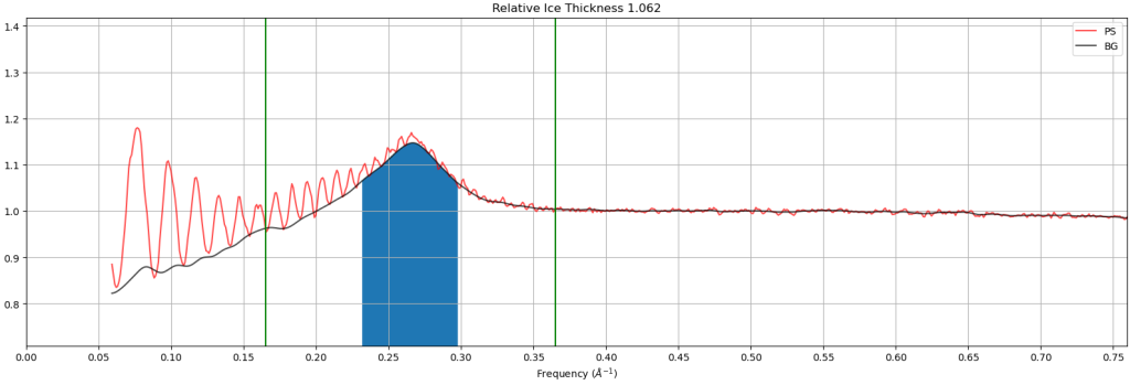
- Relative ice thickness: This plot shows the estimated relative ice thickness of a micrograph by comparing the intensity of the “water ring” at 3.6Å versus the background. In this example, the height of the water ring over the background is easily seen, indicating that this micrograph has thicker ice than micrographs that do not have a water ring. Note: This is a relative measure, not an absolute measure, making it hard to compare datasets and instruments.
Additional online content:
Hands on:
Process RELION or cryoSPARC tutorial data:
- What happens if you change the defocus search range to be smaller, like 10,000Å to 20,000Å? What does it look like for micrographs that aren’t correctly estimated by the CTF estimation program?
Interactive online resources:
Part 1C & 1D – Particle picking & extraction
Now that your data is aligned and CTF-estimated, it is time to select particles from your micrographs. Particle picking represents one of the most subjective and important steps in single particle analysis. The data are so noisy that small differences in picking parameters can lead to significantly different outcomes.
The goal of particle picking is to minimize picking “junk” (i.e., everything that is not your particle, like ice, aggregates, and noise) while maximizing picking “signal” (i.e., your particle).
Choosing a particle picking approach
There are three broad categories of particle picking:
- Shape-based – no prior information needed other than particle diameter
- Template matching – uses 2D references (class averages or 2D projections of a 3D reference)
- Neural network – uses artificial-intelligence-trained algorithms to select particles
Below, we will discuss these categories, comparing/contrasting their use and performance.
Additional online resources describing particle picking:
- CryoEM101.org – Particle picking & extraction
- Theory of CryoEM SPA. 3. Particle selection and pruning – Carlos Oscar Sánchez Sorzano
Shape-based
This approach uses an imaging filtering technique to find objects of a user-defined size. Typically, this approach will use an image processing technique known as ‘difference of Gaussians’ (or, in RELION, ‘difference of laplacians’) that allows the detection of object edges. This approach requires no prior information about the particle other than a user-specified diameter and threshold.
To give an example of what this looks like, here is an adapted figure showing what the difference of Gaussians will do to cryo-EM micrographs:
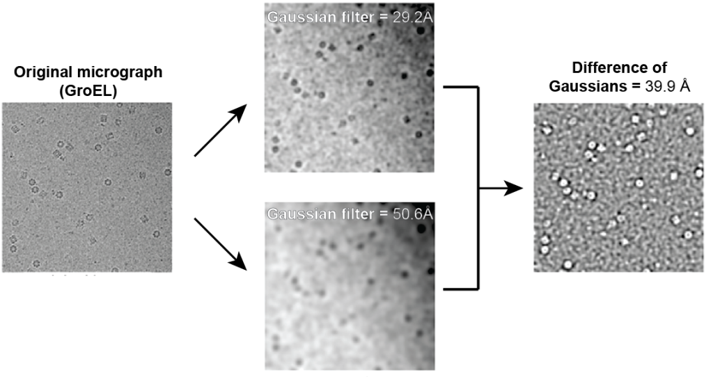
Figure reference: Voss et al. 2009
Here, you can see that the difference between the two Gaussian-filtered images leads to sharp edges of the GroEL particles. The brightness of this output Difference of the Gaussian image is then used for identifying particles – a more intense signal can be selected to identify particles.
- Typical parameters: particle diameter and threshold. Programs ask for a single diameter (or a range of possible diameters) that will be used to filter the image. Then, a user-specified threshold will be used to identify which object is a particle.
- Pros: Fast; user does not need to know the structure other than the diameter that they can measure in micrographs.
- Cons: Due to the high noise of cryo-EM datasets, this approach is prone to picking ‘junk,’ leading to a lot of false positives. False positive picks will degrade the quality of subsequent 2D class averages.
- Example job names: CryoSPARC – Blob picker; RELION – Autopicking: Laplacian of Gaussians
Primary literature
- DoG Picker and TiltPicker: software tools to facilitate particle selection in single particle electron microscopy. Voss et al. 2009 Journal of Structural Biology PMID: 19374019.
- New tools for automated high-resolution cryo-EM structure determination in RELION-3. Zivanov et al. 2018 eLife PMID: 30412051.
Template matching
In this approach, users provide 2D class averages or 3D reconstruction projections as templates for picking from a dataset. These templates are then tiled across micrographs, calculating cross-correlation scores for all template rotations. The user will then specify a score threshold, determining which scores constitute a real particle.
Here is an example of picking top and side view of keyhole limpet hemocyanin (KLH) from cryo-EM micrographs. The templates for picking are shown as insets in the images – blue arrows correspond to the side view and black arrows correspond to the top down view:
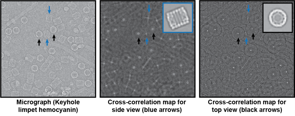
Figure reference: Roseman 2004
In this example, the resulting cross-correlation map for the inset template shows sharp, bright spots when the particle matches the template. The better the template, the sharper the peak and cross-correlation score.
- Typical inputs & parameters: Class averages or 3D projects. Note – this process is performed on binned, filtered images, so you only need 10-15 templates. Users will need to identify upper and lower score thresholds to identify what a particle is.
- Pros: This approach will be accurate if you have high-quality 2D class averages (crisp features, <9Å resolution) that represent all viewing directions of your molecule.
- Cons: Templates are required. Thus, you need to know what you are looking for in the data. Additionally, the quality of the templates will affect the particle pick quality.
- Example job names: RELION – Autopicking: Template; CryoSPARC – Template picker.
Primary literature:
- FindEM–a fast, efficient program for automatic selection of particles from electron micrographs. Roseman 2004 . Journal of Structural Biology PMID: 15065677.
- Semi-automated selection of cryo-EM particles in RELION-1.3. Scheres 2015 Journal of Structural Biology PMID: 25486611.
Neural network
In this approach, convolutional neural networks are trained and then used to select particles from micrographs. Convolutional neural networks are frameworks that allow neural networks to operate on image data, performing successive operations to extract features from image data. Importantly, all neural networks in cryo-EM must be trained either by the algorithm developers or by individual users. Training involves manually picking hundreds to thousands of particles and then feeding these picks into a convolutional neural network to learn what patterns accurately define what ‘is’ a particle. The training produces a neural network weights file, which is a file that has weights for the matrices in the convolutional network. These files can be saved and shared. For some neural network pickers, a ‘general’ picker can be trained from a diverse set of particle picks.
- Typical parameters: Parameters will vary depending on the architecture of the neural network. All will share a threshold cutoff to avoid junk.
- Pros: Once trained, neural network pickers are fast and accurate.
- Cons: Training neural networks can be cumbersome, and it can be hard to know how to improve neural network pickers if they are not performing well for a given dataset.
- Example job names: Topaz, Warp, crYOLO.
- Practical considerations:
- Topaz – No general model; requires training per sample/per dataset. Is free standing or incorporated into RELION and cryoSPARC.
- Warp – Has a general model but typically requires user re-training with specific sample types. Once trained, the neural network can work across different datasets and similar sample types. Note: Warp only runs on Windows. Warp also has a junk detector that will automatically avoid junk based on a pre-trained neural network.
- crYOLO – Has a general model that works well on most samples. Currently, is free standing or a part of the SPHIRE package.
Primary literature
- Positive-unlabeled convolutional neural networks for particle picking in cryo-electron micrographs. Bepler et al. 2019 Nature Methods PMID: 31591578.
- Real-time cryo-electron microscopy data preprocessing with Warp. Tegunov & Cramer 2019 Nature Methods PMID: 31591575.
- SPHIRE-crYOLO is a fast and accurate fully automated particle picker for cryo-EM. Wagner et al. 2019 Communications Biology PMID: 31240256.
Additional online content:
- Tristan Bepler – SBGrid Webinar: Topaz
- Dmitry Tegunov – NeCEN Webinar: Warp
- Thorsten Wagner – SBGrid Webinar: crYOLO
- National Cryo-EM Centers Webinar: Round table discussion on neural network pickers.
Selecting a box size for extracted particles
Due to the low atomic number of proteins in vitreous water, images are defocused to generate phase contrast. The effect of defocusing is the delocalization of information away from a particle. The higher the defocus, the further the information is moved from the particle.
To show what delocalized information looks like, here is an example of TRPV1:
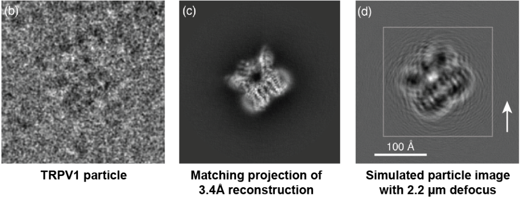
Figure reference: Sigworth 2016. Original dataset of TRPV1: Liao et al. 2013.
The left image shows a cryo-EM particle of TRPV1 aligned to the forward projection of the 3.4Å 3D reconstruction of TRPV1 (middle). Note that the projection is from a CTF-corrected 3D reconstruction (we will discuss more about CTF correction in other sections). To highlight the effect of defocus, the right image shows a simulated particle without noise at a defocus of 2.2 microns. The defocused simulated particle shows ripples far away from the actual particle, showing what defocus will do to particle information.
The white arrow shows the farthest location where ripples can be seen far away (~100Å) from the actual particle. Thus, the box size used to extract particles must consider this delocalization; otherwise, information will be missing from the particle. To highlight this effect, notice that if we extracted the TRPV1 particle using the smaller inset square in the right image, we would be missing information (i.e., the ripples) that extend past the inset box. This would result in a lower-resolution 3D reconstruction.
How do you know what box size to use?
Peter Rosenthal & Richard Henderson describe the relationship between box size, defocus, and resolution.
First, the box size, in Angstroms, is described as:
Box size = D + 2R
Where:
- R = displacement expected for average defocus
- D = particle diameter
The displacement R is defined by:
R = λΔF/d
Where:
- λ = electron wavelength
- ΔF = defocus
- d = resolution (i.e., what resolution are you interested in obtaining in your final reconstruction).
For the TRPV1 example above, the displacement of 3.4Å information away from the particle at 2.2 microns defocus and 300 kV can be calculated:
R = ( 0.0197Å * 22,000 Å ) / 3.4Å = 127Å
Box size = 100 Å diameter + 2 * 127 Å = 354 Å
Electron wavelengths (Å):
- 300 kV = 0.0197 Å
- 200 kV = 0.0257 Å
- 120 kV = 0.0335 Å
Primary literature:
- Optimal determination of particle orientation, absolute hand, and contrast loss in single-particle electron cryomicroscopy. Rosenthal & Henderson 2003 Journal of Molecular Biology PMID: 14568533.
Additional online resources:
Binning extracted particles (or not)
During particle extraction, you will have a choice of binning your particle images to large pixel sizes. Binning removes high-resolution information during alignment and speeds up image processing.
Binning particle stacks will depend on which software programs you are using:
- RELION – If you are using RELION, you must bin your particles for 2D classification. Typically, users will bin to a pixel size of ~4Å so that there is a Nyquist sampling limit of 8Å, a limit that will still allow you to see alpha-helical structural in good 2D classes. In subsequent steps in RELION, you will need to balance using binned data (faster, lower resolution) versus less binning / unbinning (slower, higher resolution). Typically, as you progress through your dataset you will progressively unbinned the data. For example, after performing multiple rounds of 2D classification with pixel size = 4Å, you might perform 3D classification using a pixel size of 2Å, and then final 3D refinements with a pixel size of 1Å.
- CryoSPARC – CryoSPARC will perform binning on the fly while processing. This means that people typically extract unbinned particle stacks and then perform binning on the fly during processing. The on-the-fly binning corresponds to resolution limits specified by particular jobs. For instance, in 2D classification there is a resolution limit (e.g., 8Å). CryoSPARC will only consider binned images of particles to this resolution.
Practical advice & guidelines
General advice:
- Particle picking is sample dependent! Try different programs to see how they work.
- Your goal is to have <20% junk picked in a given dataset. If you have >20%, you will have more noise to remove and this may affect the alignment of the ‘good’ particles.
- Inspect picking carefully to make sure you are picking all ‘kinds’ of particles. Are you picking all of the largest particles? The smallest particles? Why or why not? What if you only pick a certain type? Do you get a different outcome?
- Depending on particle density, consider removing duplicate particles after particle extraction.
CryoSPARC:
- General workflow for new samples: Blob picking > get class averages (even if they are low-ish resolution > use class averages for picking with template matching. Repeat if necessary.
- Consider training Topaz for particle picking. It will take longer to pick hundreds to thousands of particles manually but it may be worth it to have higher-quality starting picks.
RELION:
- One approach for new samples: Laplacian of Gaussians > get class averages (even if they are low-ish resolution > use class averages for picking with template matching. Repeat if necessary.
- Alternatively, you should consider trying crYOLO, which will run outside of RELION. Then you can import the picked particles into RELION.
Hands-on
Process RELION or cryoSPARC tutorial data:
- Compare an ‘overpicked’ (i.e., regions of ice also picked) vs. ‘underpicked’ (i.e., stringent, all picks are particles but you’re missing some particles). What do resulting 2D class averages look like?
- What happens if you run 2D classification with higher resolution or lower resolution data?
- RELION: Extract particle stacks at full pixel size and run 2D classification. Compare this with a run using a 4Å pixel size or an 8Å pixel size. How do the resulting averages change in appearance?
- cryoSPARC: Extract at full pixel size, but change the resolution limit during 2D classification. Try a resolution limit of 3Å versus 8Å versus 12Å. What do you notice?
Interactive online resources:
Please submit any suggestions or comments to cryoedu-support [at] umich.edu.